NTL9

To provide examples of ID applications, we used trajectories of fast folding proteins generated by D. E. Shaw group (DOI:10.1126/science.1208351).

In particular, we used N-terminal Domain of Ribosomal Protein L9 (NTL9, PDB: 2HBA(1-39)) containing a single point mutation, K12M, to increase its stability by 1.9 kcal mol⁻¹ .

We used protein structure and trajectory data of DESRES-Trajectory_NTL9-2-protein. We sampled the originally simulated trajectory in 6 shorter sub-trajectories of 2000 frames each, representing either the folded state of the protein (f0, f1, f2) or the unfolded one (u0, u1, u2).

Original Trajectory	New Trajectory	Frames	State
NTL9-2-protein-000.dcd	ntl9_u0.xtc	[:2000]	Unfolded
NTL9-2-protein-050.dcd	ntl9_f0.xtc	[:2000]	Folded
NTL9-2-protein-080.dcd	ntl9_u1.xtc	[:2000]	Unfolded
NTL9-2-protein-100.dcd	ntl9_f1.xtc	[:2000]	Folded
NTL9-2-protein-124.dcd	ntl9_u2.xtc	[:2000]	Unfolded
NTL9-2-protein-194.dcd	ntl9_f2.xtc	[:2000]	Folded

intrinsic_dimension()

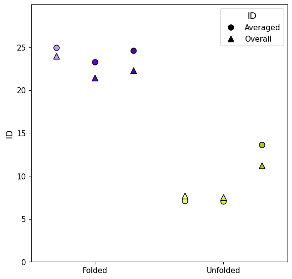
By computing ID as local it is possible to see how this value evolves along the trajectory, we called it Instantaneous ID.

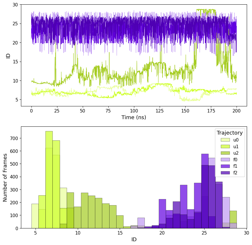
The trajectories are clearly split in two ID groups, so we can divide the trajectories in "folded" and "unfolded" by setting a threshold at ID<20, this shows the capability of ID to identify the two distinct states.

This can be done both with local (including standard deviations) ID and the mean of the global ID along the trajectory.

sections_id()

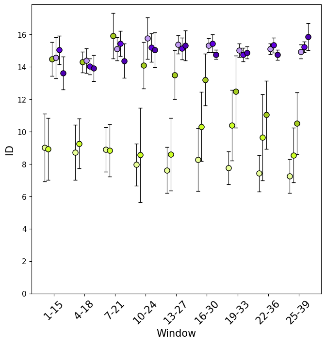
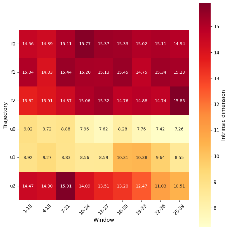
Similarly, with section_id, it is possible to visualise, for each window, the value of ID along the trajectory (both as global ID and local).

In this case it is intresting to notice how ID differs between replicas and windows, for example replica u2 completely overlaps with the folded values for the first few windows.

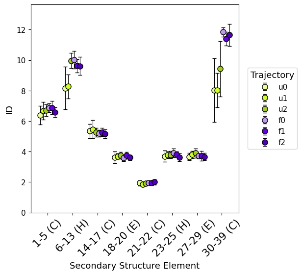
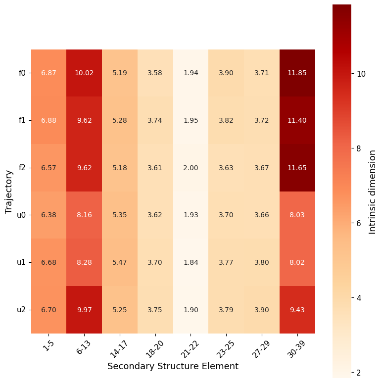
secondary_structure_id()

secondary_structure_id, divides the protein by secondary structure elements instead of same-length windows, estimating ID along the trajectory on each element individually (both as global ID and local).

Computing ID separately for each secondary structure element provides more detailed insights into the protein’s flexibility, as different types of secondary structures comprise distinct levels of flexibility in specific regions.